Monitoring Cassandra

Monitoring Challenges

We access Cassandra through our standard NoSQL proxy layer Apollo, which gives us great application level performance and availability metrics for free via our uwsgi metrics framework. This immediately gives us the capability to alert developers when their Cassandra based application is slow or unavailable. Couple these pageable events with reporting the out of the box JMX metrics on query timing to customers and the monitoring story is starting to look pretty good for consumers of Cassandra.
The main difficulty we faced was monitoring the state of the entire database for operators of Cassandra. Some of the metrics exposed over JMX are useful to operators. There are a lot of good resources online to learn which JMX metrics are most relevant to operators, so I won’t cover them here. Unfortunately, most of the advanced cluster state monitoring is built into nodetool which is useful for an operator tending to a specific cluster but does not scale well to multiple clusters with a distributed DevOps ownership model where teams are responsible for their own clusters. For example, how would one robustly integrate the output of nodetool with Nagios or Sensu? OpsCenter is closer to what we need, especially if you pay for the enterprise edition, but the reality is that this option is expensive, does not monitor ring health in the way we want and does not (yet) support 2.2 clusters.
We need to be able to determine a datastore is going to fail before it fails. Good datastores have warning signs, but it’s a matter of identifying them. In our experience, the JMX metrics monitoring technique works well when you’re having a performance or availability problem isolated to one or two nodes. The technique falls flat, however, when trying to differentiate between an innocuous single node failure impacting a keyspace with a replication factor of five and a potentially critical single node failure impacting a keyspace with a replication factor of two.

Finding Cassandra’s Warning Signs

Cassandra uses a ring topology to store data. This topology divides the database into contiguous ranges and assigns each of the ranges to a set of nodes, called replicas. Consumers query the datastore with an associated consistency level which indicates to Cassandra how many of these replicas must participate when answering a query. For example, a keyspace might have a replication factor of 3, which means that every piece of data is replicated to three nodes. When a query is issued at LOCAL_QUORUM, we need to contact at least ⅔ of the replicas. If a single host in the cluster is down, the cluster can still satisfy operations, but if two nodes fail some ranges of the ring will become unavailable.
Figure 1 is a basic visualization of how data is mapped onto a single Cassandra ring with virtual nodes. The figure elides details of datacenter and rack awareness, and does not illustrate the typically much higher number of tokens than nodes. However, it is sufficient to explain our monitoring approach.

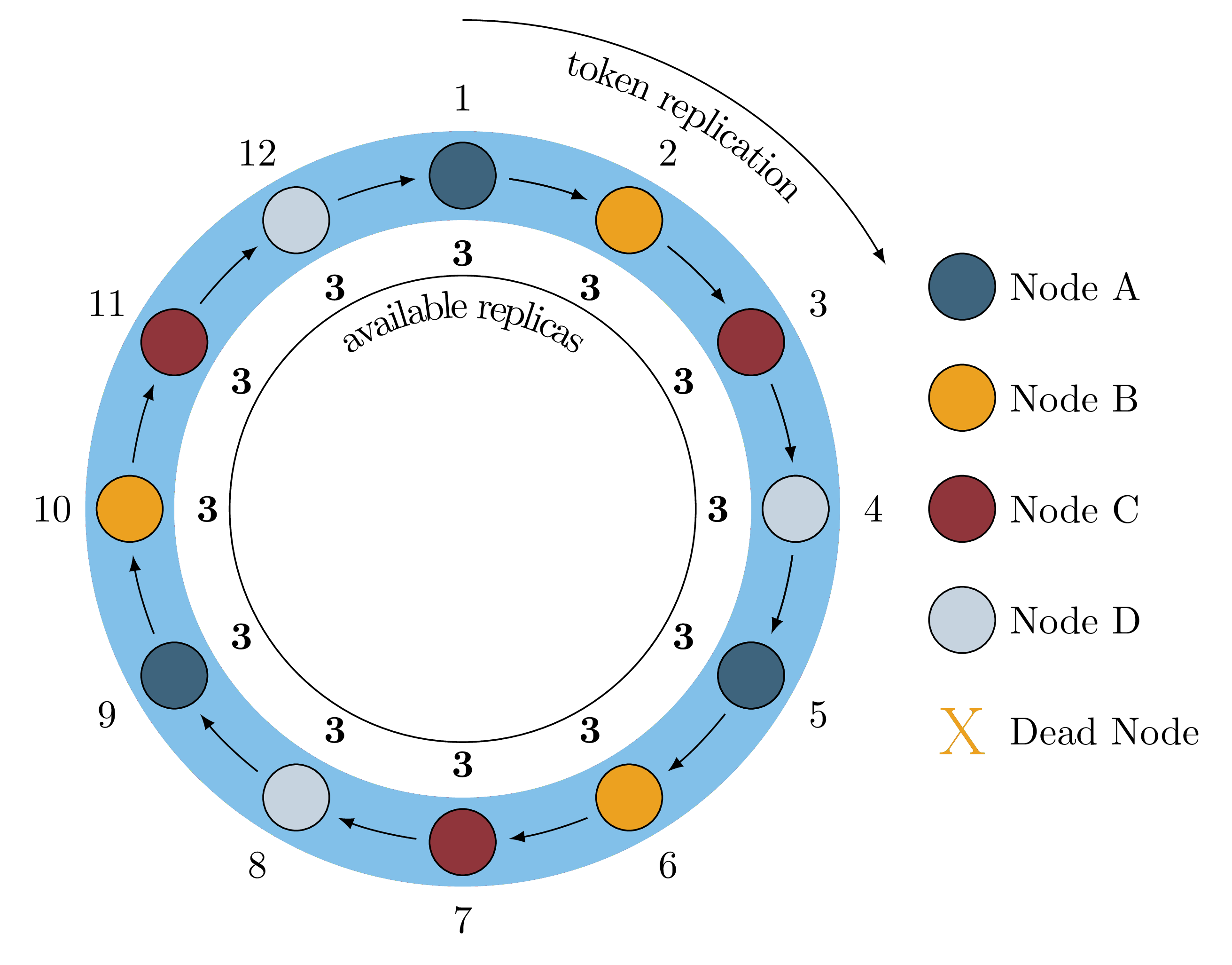
Figure 1: A Healthy Ring

In this case we have four nodes, each with three “virtual” nodes (a.k.a. vnodes ) and the keyspace has a replication factor of three. For the sake of explanation, we assume that we only have twelve ranges of data and data replicates to the three closest virtual nodes in a clockwise fashion. For example, if a key falls in token range 9, it is stored on Node A, Node B and Node C. When all physical hosts are healthy, all token ranges have all three replicas available, indicated by the threes on the inside of the ring. When a single node fails, say Node A, we lose a replica of nine token ranges because any token range that would replicate to Node A is impacted. For example, a key that would map to token range 8 would typically replicate to Node D, Node A and Node B but it cannot replicate to to Node A because Node A is down. This is illustrated in Figure 2.

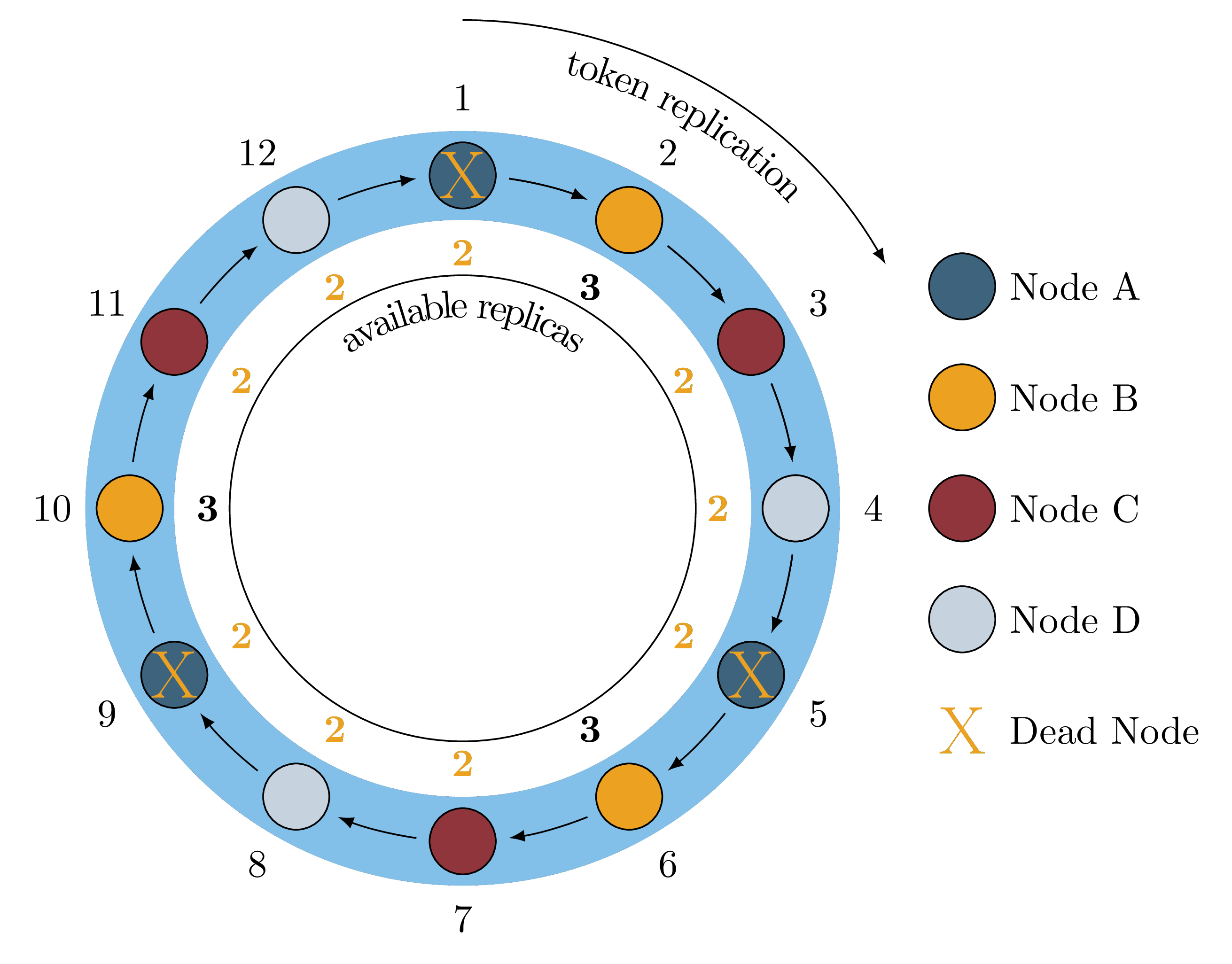
Figure 2: Single Node Failure

At this point we can still execute operations at LOCAL_QUORUM because ⅔ of replicas are still available for all token ranges, but if we were to lose another node, say Node C, we would lose a second replica of six token ranges as shown in Figure 3.

Figure 3: Two Node Failures

This means that any key which exists on those six token ranges is unavailable at LOCAL_QUORUM, while any keys not in those ranges are still available.
This understanding allows us to check if a cluster is unavailable for a particular consistency level of operations by inspecting the ring and verifying that all ranges have enough nodes in the “UP” state. It is important to note that client side metrics are not sufficient to tell if a single additional node failure will prevent queries from completing, because the client operations are binary: they either succeed or not. We can tell they are failing, but can’t see the warning signs before failure.

Monitoring Cassandra’s Warning Signs

Under the hood, nodetool uses a JMX interface to retrieve information like ring topology, so with some sleuthing in the nodetool and Cassandra source code we can find the following useful mbeans:

• type=StorageService/getRangeToEndpointMap/{keyspace}
• type=EndpointSnitchInfo/getDatacenter/{node}
• type=StorageService/Keyspaces
• type=StorageService/LiveNodes

In order to programmatically access these mbeans we install jolokia on all of our Cassandra clusters. An HTTP interface to Cassandra’s mbeans is extremely powerful for allowing quick iteration on automation and monitoring. For instance, our monitoring script can be as simple as (pseudocode):

view raw check_cassandra_pseudocode.py hosted with ❤ by GitHub

Often our applications using Cassandra read and write at LOCAL_ONE, which means that we can get robust monitoring by deploying the above check twice: the first monitoring LOCAL_ONE that pages operators, and the second monitoring LOCAL_QUORUM that cuts a ticket on operators. When running with a replication factor of three, this allows us to lose one node without alerting anyone, ticket after losing two (imminently unavailable), and page upon losing all replicas (unavailable).
This approach is very flexible because we can find the highest consistency level of any operation against a given cluster and then tailor our monitoring to check the cluster at the appropriate consistency level. For example, if the application does reads and writes at quorum we would ticket after LOCAL_ALL and page on LOCAL_QUORUM. At Yelp, any cluster owner can control these alerting thresholds individually.

A Working Example

The real solution has to be slightly more complicated because of cross-datacenter replication and flexible consistency levels. To demo this approach really works, we can setup a three node Cassandra cluster with two keyspaces, one with a replication factor of one (blog_1) and one with a replication factor of three (blog_3). In this configuration each node has the default 256 vnodes.

view raw create_keyspaces.cql hosted with ❤ by GitHub

We like to write our monitoring scripts in Python because we can integrate seamlessly with our pysensu-yelp library for emitting alerts to Sensu, but for this demo I’ve created a simplified monitoring script that inspects the ring and exits with a status code that conforms to the Nagios Plugin API. As we remove nodes we can use this script to see how we gradually lose the ability to operate at certain consistency levels. We can also check that the number of under-replicated ranges matches our understanding of vnodes and replication:

view raw testing_it_out.sh hosted with ❤ by GitHub

Now it’s just a matter of tuning the monitoring to look for one level of consistency higher than what we actually query at, and we have achieved robust monitoring!
An important thing to understand is that this script probably won’t “just work” in your infrastructure, especially if you are not using jolokia, but it may be useful as a template for writing your own robust monitoring.

Take it to 11, What’s Next?

Our SREs can sleep better at night knowing that our Cassandra clusters will give us warning before they bring down the website, but at Yelp we always ask, “what’s next?”
Once we can reliably monitor ring health, we can can use this capability to further automate our Cassandra clusters. For example, we’ve already used this monitoring strategy to enable robust rolling restarts that ensures ring health at every step of the restart. A project we’re currently working on is combining this information with autoscaling events to be able to intelligently react to hardware failure in an automated fashion. Another logical next step is to automatically deduce the consistency levels to monitor by hooking into our Apollo proxy layer and updating our monitoring from the live stream of queries against keyspaces. This way if we change the queries to a different consistency level, the monitoring follows along.
Furthermore, if this approach proves useful long term, it is fairly easy to integrate it into nodetool directly, e.g. nodetool health <keyspace> <consistency_level>.

replication_level = input(...)

alive_nodes = getLiveNodes(...)

keyspaces = getKeyspaces(...) - system_keyspaces()

underreplicated_keyspaces = {}

for keyspace in keyspace:

keyspace_ranges = getRangeToEndpointMap(keyspace)

for _, range_nodes in keyspace_ranges:

if |range_nodes ∩ alive_nodes| < replication_level:

underreplicated_keyspaces[keyspace] = True

if underreplicated_keyspaces:

alert_cluster_operator(underreplicated_keyspaces)

cqlsh:blog_1> DESCRIBE CLUSTER

Cluster: test

Partitioner: Murmur3Partitioner

Range ownership:

3732272507813644288 [NODE_A]

2788686370127196454 [NODE_B]

-7530935857429381116 [NODE_B]

111150679707998215 [NODE_B]

3524081553196673032 [NODE_A]

2388757566836860943 [NODE_B]

6174693015045179395 [NODE_A]

81565236350140436 [NODE_B]

9067682831513077639 [NODE_C]

3254554184914284573 [NODE_B]

8220009980887493637 [NODE_C]

...

cqlsh:blog_1> use blog_3 ;

cqlsh:blog_3> DESCRIBE CLUSTER

Cluster: test

Partitioner: Murmur3Partitioner

Range ownership:

3732272507813644288 [NODE_A, NODE_B, NODE_C]

2788686370127196454 [NODE_B, NODE_C, NODE_A]

-7530935857429381116 [NODE_B, NODE_C, NODE_A]

111150679707998215 [NODE_B, NODE_C, NODE_A]

3524081553196673032 [NODE_A, NODE_B, NODE_C]

2388757566836860943 [NODE_B, NODE_C, NODE_A]

6174693015045179395 [NODE_A, NODE_B, NODE_C]

...

# All nodes are running normally

# Check availability of keyspaces

(venv)$ ./check_cassandra_cluster --host NODE_A all

OK: cluster looks fine

(venv)$ ./check_cassandra_cluster --host NODE_A local_quorum

OK: cluster looks fine

# Stop NODE_A

# ...

# Check availability of keyspaces

(venv)$ ./check_cassandra_cluster --host NODE_B all

CRITICAL: cluster cannot complete operations at consistency level all.

[Underreplicated partitions: {u'blog_3': 768, u'blog_1': 256}]

(venv)$ ./check_cassandra_cluster --host NODE_B local_quorum

CRITICAL: cluster cannot complete operations at consistency level local_quorum.

[Underreplicated partitions: {u'blog_1': 256}]

(venv)$ ./check_cassandra_cluster --host NODE_B local_one

CRITICAL: cluster cannot complete operations at consistency level local_one.

[Underreplicated partitions: {u'blog_1': 256}]

# Stop NODE_B as well

# ...

# Check availability of keyspaces

(venv)$ ./check_cassandra_cluster --host NODE_C all

CRITICAL: cluster cannot complete operations at consistency level all.

[Underreplicated partitions: {u'blog_3': 768, u'blog_1': 512}]

(venv)$ ./check_cassandra_cluster --host NODE_C local_quorum

CRITICAL: cluster cannot complete operations at consistency level local_quorum.

[Underreplicated partitions: {u'blog_3': 768, u'blog_1': 512}]

(venv)$ ./check_cassandra_cluster --host NODE_C local_one

CRITICAL: cluster cannot complete operations at consistency level local_one.

[Underreplicated partitions: {u'blog_1': 512}]

Cluster Name Change

Cluster name change

Follow these steps to update the name of the cluster on a single node:

Step 1 - While the node is up, update the cluster name in the database as follows:

cqlsh> UPDATE system.local SET cluster_name = 'ITF Cluster' where key='local';

NOTE: If there are multiple nodes, remember to perform this step on each node as this only updates the node's local system table.

Step 2 - Update the value of cluster_name: in cassandra.yaml.

Step 3 - Prepare for a clean shutdown:

$ nodetool flush

$ nodetool drain

Step 4 - Restart DSE.

Step 5 - If using OpsCenter, restart opscenterd on the OpsCenter server for the name change to be recognised.

Cassandra Storage Sizing

Column Overhead and Sizing

Every column in a ColumnFamily requires overhead.  And since every row can contain different column names as well as a different number of columns, the column meta-data must be stored with every row.

For every column, the following must be saved:

name : 2 bytes (len as short int) + byte[]

flags : 1 byte

if counter column : 8 bytes (timestamp of last delete)

if expiring column : 4 bytes (TTL) + 4 bytes (local deletion time)

timestamp : 8 bytes (long)

value : 4 bytes (len as int) + byte[]

For the majority of us (the ones not using TTL or Counters) the formula would be:

Ø  Column size = 15 + size of name + size of value

This tells us that if you have columns with small values, the column metadata can account for a non-trivial part of your storage requirements.  For example let's say you are using a timestamp (long) for column name and another long for the column value.  Using the formula:

column size = 15 + 8 + 8 = 31 bytes.  23 (bytes of overhead to store 8 bytes of data!)

See org.apache.cassandra.db.ColumnSerializer for more details.

Row Overhead and Sizing

Just like columns, every row incurs some overhead as well when stored on disk in an SSTABLE.  As you can see below, I don't have values for the bloom filter nor index overhead.  Calculating them is proportional to the size of the row and number of columns.  I'll give a rough estimate for both of them, but I don't completely understand bloom filters, so forgive me.  For every row, the following is stored:

key : 2 bytes (len as short) + byte[]

flag : 1 byte (1 or 0)

ColumnFamily ID : 4 bytes (int)

local deletion time : 4 bytes (int)

marked for delete time : 8 bytes (long)

column count : 4 bytes (int)

data : all columns (overhead + data)

row bloom filter : ???

row index : ???

As you can see there is a lot going on when storing a row of columns!  Minimally there are 26 bytes of overhead (including minimum size for bloom filter.)  It is basically impossible to predict the actual row size if your key size varies or your column data size varies.  So best just to pick some averages for key size, number of columns, etc and get an estimate:

Ø  row overhead = 23 + avg key size + bloom filter size + index size

Bloom Filter Size

The bloom filter is complicated and the following formula is only an estimate, but should capture the majority of use cases … if I understand things correctly:

Ø  bloom filter size = 2 bytes (len as short) + (8 + ceiling((number of columns * 4 + 20) / 8))

Example:  if you have 40 columns, then the bloom filter will require ~33 bytes.

For a row with only a few columns and not much data the size of the bloom filter seems more significant than a row with many columns.

See org.apache.cassandra.utils.BloomFilter and org.apache.cassandra.utils.BloomFilterSerializer for more details.

Index Size

The row index helps optimize locating a specific column within a row.  The size of the index will normally be zero unless you have rows with a lot of columns and/or data.  For the index size to grow larger than zero, the size of the row (overhead + column data) must exceed column_index_size_in_kb, defined in your YAML file (default = 64.)  If the size is exceeded, one index entry is created for each column_index_size_in_kb number of bytes in the row.  So if your row is 80kb, there will be two index entries.

An index entry consists of:

first col name : 2 bytes + byte[]

last col name : 2 bytes + byte[]

offset into the row data : 8 bytes (long)

width of data : 8 bytes (long)

The formulat for calculating number of index entries:

Ø  number of entries = ceiling(row data size / column_index_size_in_kb)

The formula for calculating size of index an index entry:

Ø  entry size = 20 + first size + last size

Each entry will be a different size if your column names differ in size, so you must calculate an average column name size for sizing the row like this:

Ø  row index size = 4 bytes [len as int] + if index size > 1 => (20 + 2 * avg name size) * numEntries

So if you have 80kb worth of data in a row and the avg column name size is 10, then the index will require the following space:

number of entries = ceiling(80kb / 64kb) = 2

row index size = 4 + (20 + 2 * 10) * 2

row index size = 84 bytes

And if you have 23kb worth of data in a row and the avg column name size is 10, then the index will require the following space (notice that the length of the index is always saved which requires 4 bytes):

number of entries = ceiling(23kb / 64kb) = 1

row index size = 4 + 0

row index size = 4 bytes

As you can see the size of the index isn't that large compared to the size of the row for default settings.  Since it is only created if the size of the row exceeds column_index_size_in_kb, most of us do not incur the overhead of the index.  And you probably should not care about it unless you have a lot of rows with a large number of columns, and/or have reduced the column_index_size_in_kb setting.

See org.apache.cassandra.io.sstable.IndexHelper for more details. 

SSTABLE Overhead and Sizing

Every SSTABLE has a Data file that contains the actual column data.  Also there is an Index, Bloom Filter, and Statistics data associated with it - each stored in its on file separate from the row data.  The size of each of these is determined by the number of rows and the key size.

Index Overhead

The index is for quickly finding where in an SSTABLE the key and its data are located.  For an index there is one entry per row key:

Row key	2 bytes (length) + byte[]
File offset into Data file	8 bytes (long)

So the index size is dependent on the number of rows and size of your keys.  For sizing purposes, just pick an average key size:

Ø  index size = rows * (10 + avg key size)

There is also a summary index and segment boundary markers, but they are not worth calculating - and I didn't want to figure it out ;)  What we can surmise from this is that the index overhead is not tiny but will only be significant if you have very narrow and skinny rows.

Bloom Filter Overhead

Bloom filters are used to quickly determine if an SSTABLE contains a key.  The bloom filter for SSTABLES is calculated similar to rows, but has a different target.  Otherwise the same code applies.  As I mentioned earlier, I am not that familiar with the bloom filter algorithm and this is just an approximation for sizing:

Ø  bloom filter size = (numRows * 15 + 20) / 8

The same can be surmised for bloom filters as the indices, if you have lots of narrow and skinny rows then the overhead for the bloom filter will be more significant.

Statistics Overhead

Very very minimal and not worth calculating.

See org.apache.cassandra.io.sstable.SSTableWriter for more details.

Replication Overhead

Replication will obviously play a role in how much storage is used.  If you set ReplicationFactor (RF) = 1 then there isn't any overhead for replicas (because you don’t have any.)  However if RF > 1 then your total data storage requirement will include replication overhead:

Ø  replication overhead = (base storage) * (RF-1)

                                          

"base storage" is based on all the calculations we've made in the previous sections – see the summary table below.

Snapshots

On linux, snapshots are made by creating hard links (man ln) to all of the data files.  By definition a hard link cannot be made across logical volumes, so the snapshots will exist on the same volume as your data files. This is very fast and does not count against storage usage until SSTABLES are removed leaving only the snapshot reference to the files.  So you can either do nothing (consuming disk space), or move them off to another volume.

If you choose to keep them on the same volume, then make sure you take into account the size of a snapshot, which is the same size as your total storage requirement.

More Overhead!

So it seems all I can talk about is overhead overhead overhead.  Well there is (at least) one more place Cassandra uses storage, during compaction.  When Cassandra performs a compaction (major or minor type) it combines a subset of existing SSTABLES into one new SSTABLE.  During the process Cassandra will discard tombstoned data and merge rows.  How much extra space is required?  Up to the total required storage size we’ve calculated thus far.  That means that you need an _additional_ “total storage” size.  If there are tombstones that can be cleared, then the extra storage will be less depending on how often you delete data.  Once the process is completed the original SSTABLES are marked as compacted and will be removed during the next GC or Cassandra restart.

Ø  Extra space for compaction = an additional "total storage” size

Example:  Suppose compaction is combining 4 SSTABLES 1gb each.  If there are no tombstones, the process will require 4gb of extra space.

Storage Sizing Summary

The following table clearly defines and summarizes the formulas from previous sections:

Number of Rows	NR	Estimated or Target number of rows in your ColumnFamily
Number of Columns Per Row	NC	Estimated/Average number of columns per row
Total Number of Columns	TNC	Number of columns in ColumnFamily
Column name size	CNS	Average size of name of column
Column value size	CVS	Average size of data stored in a column value
Row key size	RKS	Average size of keys
ReplicationFactor	RF
Number of Nodes	NN	Number of nodes in cluster
Column data	NR * NC * CVS
Column overhead	NR * NC * (15 + CNS)
Column overhead (counter)	NR * NC * (23 + CNS)
Column overhead (w/TTL)	NR * NC * (19 + CNS)
Row header overhead	NR * (23 + RKS)
Row bloom filter	NR * (2 bytes (len as short) + (8 + ceiling((NC * 4 + 20) / 8)))
Row index	4 bytes [len as int] + if index size > 1 => (20 + 2 * avg name size) * numEntries	Number of entries in index is always written.  See above for more details
SSTABLE index	NR * (10 + RKS)
SSTABLE bloom filter	(NR * 15 + 20)/8
Base Storage	BS	Sum of everything above
Additional Replicas	BS * (RF-1)
Compaction Overhead	BS * RF
Total Storage	BS * RF * 2
Snapshots	Total Storage	For every snapshot, “Total Storage” space is required.  Remember to move them off the data volume and you will recover the space

Every column requires overhead that cannot be overlooked

For sizing purposes just assume your column names are 10 bytes each, so the total overhead per column is 15 + 10 = 25 bytes.   That's just the overhead, don't forget about the actual size of the values.  It's the ratio of the data size to the overhead that surprises people.  If you have a lot of columns with small data sizes you will very likely have more overhead than actual data.

Compaction overhead requires enough space for an additional copy of the data

This figure assumes no deletes.  This is a _LARGE_ requirement which is being optimized in a future Cassandra release.

Use Case where overhead far exceeds data size

Let's say we want to save the the number of times per day that a URL on our website has been accessed.  And we’ll assume that over time, 1 million URLs will be accessed on average about 10 different days per URL.

NR	1,000,000	Estimated or Target number of rows in your ColumnFamily
NC	10	Average over all the rows
TNC	10,000,000	Total number of columns
CNS	8	All names are timestamps (long)
CVS	4	All values are counts (integer)
RKS	50	Average URL length
RF	3	Replication Factor
Number of Nodes	9

We will have the following space requirement:

Column data	1,000,000 * 10 * 4	40mb
Column overhead	1,000,000 * 10 * (15+8)	230mb
Row header overhead	1,000,000 * (23 + 50 + 0)	73mb
Row bloom filter	1,000,000 * (2+8 + ceiling((10 * 4 + 20) / 8))	18mb
Row index	RI = 1,000,000 * 4	4mb We assume no indices because it will require 2,428 days to exceed the default column_index_size_in_kb limit.
SSTABLE index	1,000,000 * (10 + 50)	60mb
SSTABLE bloom filter	(1,000,000 * 15 + 20)/8	1.9mb
Base Storage	BS	426,875,003 = ~427mb
Additional Replicas	427mb * (3-1)	853,750,005 = ~854mb
Compaction Overhead	427mb * 3	1,280,625,008 = ~1,281mb
Total Storage	427mb * 3 * 2	2,561,250,015 = ~2,561mb

                                                                                                                   

Actual column value data = 40mb (9.4%)

Column overhead = 230mb (53.9%)

Row overhead = 95mb (22.2%)

SSTABLE overhead = 61.9mb (14.5%)

Summary

So you can see that in the example Use Case the overhead is over 9 times the actual data size!  This doesn’t mean the overhead is bad or should be reduced.  In this case the column names do more than simply designate a value, they actually store the timestamp (date) when the URL was accessed.  This exercise is merely to determine your required storage footprint and allow you to plan for the future.

Enjoy